Download the notebook here!

Maximum Likelihood Estimation

Estimagic has a special interface to estimate model parameters via maximum likelihood. We take a look at the same ordered logit model from the more general optimization tutorial.

data = pd.read_pickle("ologit.pickle")
formula = 'apply ~ pared + public + gpa'
estimates = ordered_logit(formula, data)

The example is taken from the Stata Documentation. The correct parameters for this model are [1.047664, -.0586828, .6157458, 2.203323,  4.298767]

import numpy as np
import pandas as pd
from scipy import stats
from estimagic.estimation.estimate import maximize_log_likelihood
from ordered_logit import ordered_logit_processing

Process the user input

To process the input for the ordered logit function, this tutorial uses ordered_logit_processing which is explained in the the more general optimization tutorial.

Calculate the Likelihood

Next we have to evaluate the likelihood function, given parameters and data. There are more efficient ways of calculating the likelihood for an ordered logit, but this one was chosen for brevity and readability.

In most optimization problem, the criterion function returns a scalar. To use the estimagic’s likelihood estimation interface, the criterion function needs to return the log likelihood contributions of observations. This has two advantages:

1. The log likelihood contributions are necessary to compute the Jacobians or Hessians for standard error calculations. Estimagic will aggregate the contributions depending on the calculation and the user only needs to specify one criterion function for all purposes.

2. It is generally encouraged to compute the log likelihood because of its numerical properties. It makes it easier to avoid under- and overflows. See also the logsumexp trick.

def ordered_logit_loglikeobs(params, y, x):
    """Likelihood function of an orderd logit model."""
    # parse the parameter vector into its quantities
    beta = params.loc["beta", "value"].to_numpy()
    cutoffs = params.loc["cutoff", "value"].to_numpy()

    # calculate deterministic part of utilities
    xb = x.dot(beta)

    # evaluate likelihood
    upper_cutoffs = np.hstack([cutoffs, np.inf])[y]
    lower_cutoffs = np.hstack([-np.inf, cutoffs])[y]
    upper_cdf = stats.logistic.cdf(upper_cutoffs - xb)
    lower_cdf = stats.logistic.cdf(lower_cutoffs - xb)

    return np.log(upper_cdf - lower_cdf)

The ordered_logit command

The estimation command follows the same patter as the maximize or minimize. Thus, nothing has to be changed except for the criterion function to adopt the other interface.

def ordered_logit(formula, data, dashboard=False):
    """Estimate an ordered probit model with maximum likelihood.

    Args:
        formula (str): A patsy formula
        data (str): A pandas DataFrame
        dashboard (bool): Switch on the dashboard.

    Returns:
        res: optimization result.

    """
    params, y, x, constr = ordered_logit_processing(formula, data)

    res = maximize_log_likelihood(
        log_like_obs=ordered_logit_loglikeobs,
        params=params,
        algorithm='scipy_L-BFGS-B',
        constraints=constr,
        criterion_kwargs={"y": y, "x": x},
        dashboard=dashboard)
    return res

Note that maximize_log_likelihood automatically uses the maximize function, so you don’t have to switch the sign of your objective function!

Use the command

df = pd.read_pickle("ologit.pickle")
form = "apply ~ pared + public + gpa"

info, params = ordered_logit(form, df, dashboard=False)

params["correct"] = [1.047664, -.0586828, .6157458, 2.203323,  4.298767]
params[["value", "correct"]]

		value	correct
type	name
beta	pared	1.047663	1.047664
	public	-0.058697	-0.058683
	gpa	0.615885	0.615746
cutoff	0	2.203830	2.203323
	1	4.299396	4.298767

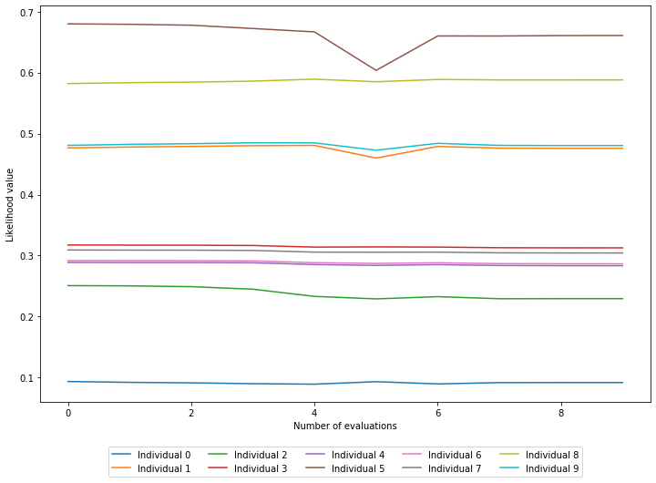
Visualizing the optimization

Estimagic does not only log parameters and criterion values in the database, but also the contributions by default. Here we are showing the contributions from the first and last evaluation to show their development. Unfortunately, this step is a little bit inconvenient for now, but will become a part of the dashboard soon.

Without much explanation, here are the likelihood contributions of ten individuals over the course of the optimization.

%matplotlib inline

import io
import pickle
import matplotlib.pyplot as plt

from estimagic.logging.create_database import load_database
from estimagic.logging.read_database import read_last_iterations

database = load_database("logging.db")
db_dump = read_last_iterations(database, ["comparison_plot"], 10, "list")
log_contributions = np.column_stack([pickle.load(io.BytesIO(i[1])) for i in db_dump[1:]])

fig, ax = plt.subplots(figsize=(12, 8))

for i in range(10):
    ax.plot(np.exp(log_contributions[i]), label=f"Individual {i}")

ax.set_xlabel("Number of evaluations")
ax.set_ylabel("Likelihood value")

ax.legend(loc="upper center", bbox_to_anchor=(0.5, -0.10), ncol=5)

plt.show()
plt.close()