import estimagic as em
import numpy as np
import pandas as pd
Numerical optimization#
Using simple examples, this tutorial shows how to do an optimization with estimagic. More details on the topics covered here can be found in the how to guides.
Basic usage of minimize#
def sphere(params):
    return params @ params
res = em.minimize(
    criterion=sphere,
    params=np.arange(5),
    algorithm="scipy_lbfgsb",
)

res.params.round(5)
array([ 0., -0., -0., -0., -0.])
params do not have to be vectors#
In estimagic, params can by arbitrary pytrees. Examples are (nested) dictionaries of numbers, arrays and pandas objects.
def dict_sphere(params):
    return params["a"] ** 2 + params["b"] ** 2 + (params["c"] ** 2).sum()
res = em.minimize(
    criterion=dict_sphere,
    params={"a": 0, "b": 1, "c": pd.Series([2, 3, 4])},
    algorithm="scipy_powell",
)

res.params
{'a': -6.821706323446569e-25,
 'b': 2.220446049250313e-16,
 'c': 0    8.881784e-16
 1    8.881784e-16
 2    1.776357e-15
 dtype: float64}
The result contains all you need to know#
res = em.minimize(
    criterion=dict_sphere,
    params={"a": 0, "b": 1, "c": pd.Series([2, 3, 4])},
    algorithm="scipy_neldermead",
)
res
Minimize with 5 free parameters terminated successfully after 805 criterion evaluations and 507 iterations.

The value of criterion improved from 30.0 to 1.6760003634613059e-16.

The scipy_neldermead algorithm reported: Optimization terminated successfully.

Independent of the convergence criteria used by scipy_neldermead, the strength of convergence can be assessed by the following criteria:

                             one_step     five_steps
relative_criterion_change  1.968e-15***  2.746e-15***
relative_params_change     9.834e-08*    1.525e-07*
absolute_criterion_change  1.968e-16***  2.746e-16***
absolute_params_change     9.834e-09**   1.525e-08*

(***: change <= 1e-10, **: change <= 1e-8, *: change <= 1e-5. Change refers to a change between accepted steps. The first column only considers the last step. The second column considers the last five steps.)
You can visualize the convergence#
fig = em.criterion_plot(res, max_evaluations=300)
fig.show(renderer="png")
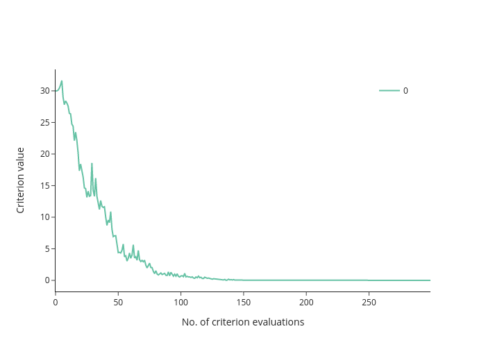
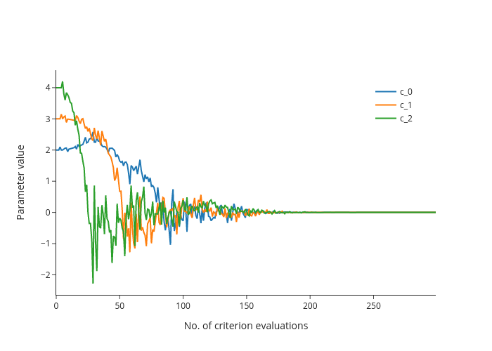
fig = em.params_plot(
    res,
    max_evaluations=300,
    # optionally select a subset of parameters to plot
    selector=lambda params: params["c"],
)
fig.show(renderer="png")
There are many optimizers#
If you install some optional dependencies, you can choose from a large (and growing) set of optimization algorithms – all with the same interface!
For example, we wrap optimizers from scipy.optimize, nlopt, cyipopt, pygmo, fides, tao and others.
We also have some optimizers that are not part of other packages. Examples are a parallel Nelder-Mead algorithm, The BHHH algorithm and a parallel Pounders algorithm.
See the full list [here](../how_to_guides/optimization/how_to_specify_algorithm_and_algo_options
You can add bounds#
res = em.minimize(
    criterion=sphere,
    params=np.arange(5),
    algorithm="scipy_lbfgsb",
    lower_bounds=np.arange(5) - 2,
    upper_bounds=np.array([10, 10, 10, np.inf, np.inf]),
)

res.params.round(5)
array([0., 0., 0., 1., 2.])
You can fix parameters#
res = em.minimize(
    criterion=sphere,
    params=np.arange(5),
    algorithm="scipy_lbfgsb",
    constraints=[{"loc": [1, 3], "type": "fixed"}],
)

res.params.round(5)
array([0., 1., 0., 3., 0.])
Or impose other constraints#
As an example, let’s impose the constraint that the first three parameters are valid probabilities, i.e. they are between zero and one and sum to one:
res = em.minimize(
    criterion=sphere,
    params=np.array([0.1, 0.5, 0.4, 4, 5]),
    algorithm="scipy_lbfgsb",
    constraints=[{"loc": [0, 1, 2], "type": "probability"}],
)

res.params.round(5)
array([ 0.33334, 0.33333, 0.33333, -0. , 0. ])
For a full overview of the constraints we support and the corresponding syntaxes, check out the documentation.
Note that "scipy_lbfgsb" is not a constrained optimizer. If you want to know how we achieve this, check out the explanations.
There is also maximize#
If you ever forgot to switch back the sign of your criterion function after doing a maximization with scipy.optimize.minimize, there is good news:
def upside_down_sphere(params):
    return -params @ params
res = em.maximize(
    criterion=upside_down_sphere,
    params=np.arange(5),
    algorithm="scipy_bfgs",
)

res.params.round(5)
array([ 0., -0., -0., 0., -0.])
estimagic got your back.
You can provide closed form derivatives#
def sphere_gradient(params):
    return 2 * params
res = em.minimize(
    criterion=sphere,
    params=np.arange(5),
    algorithm="scipy_lbfgsb",
    derivative=sphere_gradient,
)
res.params.round(5)
array([ 0., -0., -0., -0., -0.])
Or use parallelized numerical derivatives#
res = em.minimize(
    criterion=sphere,
    params=np.arange(5),
    algorithm="scipy_lbfgsb",
    numdiff_options={"n_cores": 6},
)

res.params.round(5)
array([ 0., -0., -0., -0., -0.])
Turn local optimizers global with multistart#
res = em.minimize(
    criterion=sphere,
    params=np.arange(10),
    algorithm="scipy_neldermead",
    soft_lower_bounds=np.full(10, -5),
    soft_upper_bounds=np.full(10, 15),
    multistart=True,
    multistart_options={"convergence.max_discoveries": 5},
)
res.params.round(5)
array([ 0., 0., -0., -0., 0., -0., 0., -0., -0., -0.])
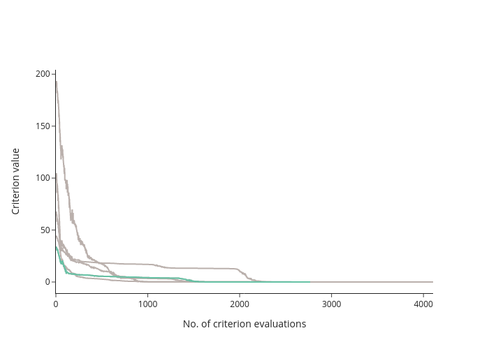
And plot the criterion history of all local optimizations#
fig = em.criterion_plot(res)
fig.show(renderer="png")
Exploit the structure of your optimization problem#
Many estimation problems have a least-squares structure. If so, specialized optimizers that exploit this structure can be much faster than standard optimizers. Likewise, other problems might have, if not a least-squares structure, at least a sum-structure (e.g. likelihood functions) that can also be exploited by suitable optimizers.
If you define your criterion function a bit differently, you can seamlessly switch between least-squares, sum-structure and standard optimizers.
def general_sphere(params):
    contribs = params**2
    out = {
        # root_contributions are the least squares residuals.
        # if you square and sum them, you get the criterion value
        "root_contributions": params,
        # if you sum up contributions, you get the criterion value
        "contributions": contribs,
        # this is the standard output
        "value": contribs.sum(),
    }
    return out
res = em.minimize(
    criterion=general_sphere,
    params=np.arange(5),
    algorithm="pounders",
)
res.params.round(5)
array([ 0., 0., -0., 0., -0.])
Using and reading persistent logging#
For long-running and difficult optimizations, it can be worthwhile to store the progress in a persistent log file. You can do this by providing a path to the logging argument:
res = em.minimize(
    criterion=sphere,
    params=np.arange(5),
    algorithm="scipy_lbfgsb",
    logging="my_log.db",
    log_options={"if_database_exists": "replace"},
)
You can read the entries in the log file (while the optimization is still running or after it has finished) as follows:
reader = em.OptimizeLogReader("my_log.db")
reader.read_history().keys()
dict_keys(['params', 'criterion', 'runtime'])
For more information on what you can do with the log file and LogReader object, check out the logging tutorial
The persistent log file is always instantly synchronized when the optimizer tries a new parameter vector. This is very handy if an optimization has to be aborted and you want to extract the current status. It is also used by the estimagic dashboard.
Customize your optimizer#
Most algorithms have a few optional arguments. Examples are convergence criteria or tuning parameters. You can find an overview of supported arguments here.
algo_options = {
    "convergence.relative_criterion_tolerance": 1e-9,
    "stopping.max_iterations": 100_000,
}

res = em.minimize(
    criterion=sphere,
    params=np.arange(5),
    algorithm="scipy_lbfgsb",
    algo_options=algo_options,
)
res.params.round(5)
array([ 0., -0., -0., -0., -0.])